Note
This example notebook demonstrates NSphere visualization techniques. The original notebook can be found in the examples directory of the NSphere project.
Copyright 2025 Marc Kamionkowski and Kris Sigurdson. Licensed under Apache-2.0 (http://www.apache.org/licenses/LICENSE-2.0).
This notebook demonstrates visualization and analysis of anisotropic velocity distributions in self-interacting dark matter halos. It reproduces all figures from the paper “Gravothermal collapse of self-interacting dark-matter halos with anisotropic velocity distributions.”
You must have successfully installed NSphere by following the instructions in the main README. Ensure the nsphere Python virtual environment is activated (source ./activate_nsphere from the project root).
This Jupyter notebook is set up to be run from the NSphere-SIDM/examples subdirectory.
Anisotropic SIDM Halo Analysis
Data Generation Commands
This notebook requires simulation data generated with the following commands from the NSphere-SIDM directory:
Constant-β models (5 runs for Figure 1, Figure 2):
# Beta = 0 (isotropic)
./nsphere \
  --ntimesteps   6250001 \
  --nout         250 \
  --dtwrite      25000 \
  --tfinal       300 \
  --profile      hernquist \
  --scale-radius 1.18 \
  --halo-mass    2.818e8 \
  --sort         6 \
  --master-seed  42 \
  --sidm \
  --tag          beta0.0

# Beta = 0.5 (radial)
./nsphere \
  --ntimesteps   6250001 \
  --nout         250 \
  --dtwrite      25000 \
  --tfinal       300 \
  --profile      hernquist \
  --scale-radius 1.18 \
  --halo-mass    2.818e8 \
  --sort         6 \
  --master-seed  42 \
  --sidm \
  --tag          beta0.5 \
  --aniso-beta   0.5
Additional runs use --aniso-beta -0.5 (tag beta-0.5), --aniso-beta -0.25 (tag beta-0.25), and --aniso-beta 0.25 (tag beta0.25) with the same parameters.
Osipkov-Merritt models (11 runs for Figure 3):
# Example: Beta(r_s) = 0.25 (extended run)
./nsphere \
  --ntimesteps      9375001 \
  --nout            375 \
  --dtwrite         25000 \
  --tfinal          450 \
  --profile         hernquist \
  --scale-radius    1.18 \
  --halo-mass       2.818e8 \
  --sort            6 \
  --master-seed     42 \
  --sidm \
  --tag             betascale0.25 \
  --aniso-betascale 0.25
Additional runs with --aniso-betascale: 0.05, 0.10, 0.15, 0.175, 0.40, 0.50, 0.60, 0.70 use the same extended parameters with corresponding tags. The isotropic run and β(r_s)=0.80 use standard parameters (tfinal=300, nout=250, ntimesteps=6250001).
Figure 4 requires no simulation data (analytical calculations only).
For more information on NSphere, see the full documentation.
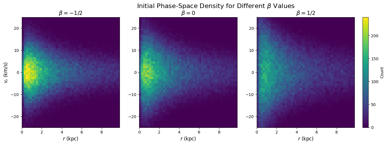
Figure 1: Initial Phase-Space Distributions for Different β Values
This cell creates the 3-panel phase-space comparison showing how the initial radial velocity distribution changes with anisotropy parameter β.
[1]:
# Import necessary libraries
import numpy as np
import matplotlib.pyplot as plt
from scipy.ndimage import gaussian_filter
from scipy.integrate import quad
import os

# Define the record dtype for binary data files
record_dtype = np.dtype([
    ('rank',  np.int32),
    ('mass',  np.float32),
    ('R',     np.float32),
    ('Vrad',  np.float32),
    ('PsiA',  np.float32),
    ('E',     np.float32),
    ('L',     np.float32)
])

# Define the paths to initial condition files for each beta value
paths = {
    r'$\beta=-1/2$': "../data/Rank_Mass_Rad_VRad_unsorted_t00000_beta-0.5_100000_6250001_300.dat",
    r'$\beta=0$': "../data/Rank_Mass_Rad_VRad_unsorted_t00000_beta0.0_100000_6250001_300.dat",
    r'$\beta=1/2$': "../data/Rank_Mass_Rad_VRad_unsorted_t00000_beta0.5_100000_6250001_300.dat"
}

# Define bin edges for radius (R) and radial velocity (Vrad)
bin_edges_R = np.arange(0, 10, 0.2)      # 0 to 10 kpc in steps of 0.2
bin_edges_V = np.arange(-50, 50, 1)      # -50 to 50 km/s in steps of 1

# Storage for histograms
histograms = {}

# Process each file
for label, file_path in paths.items():
    try:
        alldata = np.fromfile(file_path, dtype=record_dtype)
        data_R = alldata['R']
        data_Vrad = alldata['Vrad'] / 1.023e-3  # Convert to km/s

        # Compute 2D histogram
        hist, _, _ = np.histogram2d(data_R, data_Vrad, bins=[bin_edges_R, bin_edges_V])
        smoothed_hist = gaussian_filter(hist, sigma=(0.1, 0.1))
        histograms[label] = smoothed_hist

    except Exception as e:
        print(f"Error reading file {file_path}: {e}")
        histograms[label] = np.zeros((len(bin_edges_R)-1, len(bin_edges_V)-1))

# Create the 3-panel figure
vmax = 240  # Match paper scale
fig, axes = plt.subplots(1, 3, figsize=(18, 5))

for idx, (label, hist) in enumerate(histograms.items()):
    ax = axes[idx]
    im = ax.imshow(hist.T, origin='lower',
                   extent=[bin_edges_R[0], bin_edges_R[-1], bin_edges_V[0], bin_edges_V[-1]],
                   aspect='auto', cmap='viridis', vmin=0, vmax=vmax)

    ax.set_xlabel(r"$r$ (kpc)", fontsize=12)
    if idx == 0:
        ax.set_ylabel(r"$v_r$ (km/s)", fontsize=12)
    ax.set_title(label, fontsize=14)
    ax.set_ylim([-25, 25])

# Add title and colorbar BEFORE tight_layout
fig.suptitle(r"Initial Phase-Space Density for Different $\beta$ Values", fontsize=16, y=0.98)
fig.colorbar(im, ax=axes.ravel().tolist(), label="Count", pad=0.02)

# Save Figure 1 as PDF (matching paper figure)
# This generates pdf/fig1.pdf - the initial phase-space density plot
# Comment out the lines below if you only want to view the figure without saving
os.makedirs("pdf", exist_ok=True)
plt.savefig("pdf/fig1.pdf", dpi=300, bbox_inches='tight')
print('Saved: pdf/fig1.pdf')

plt.show()
Saved: pdf/fig1.pdf
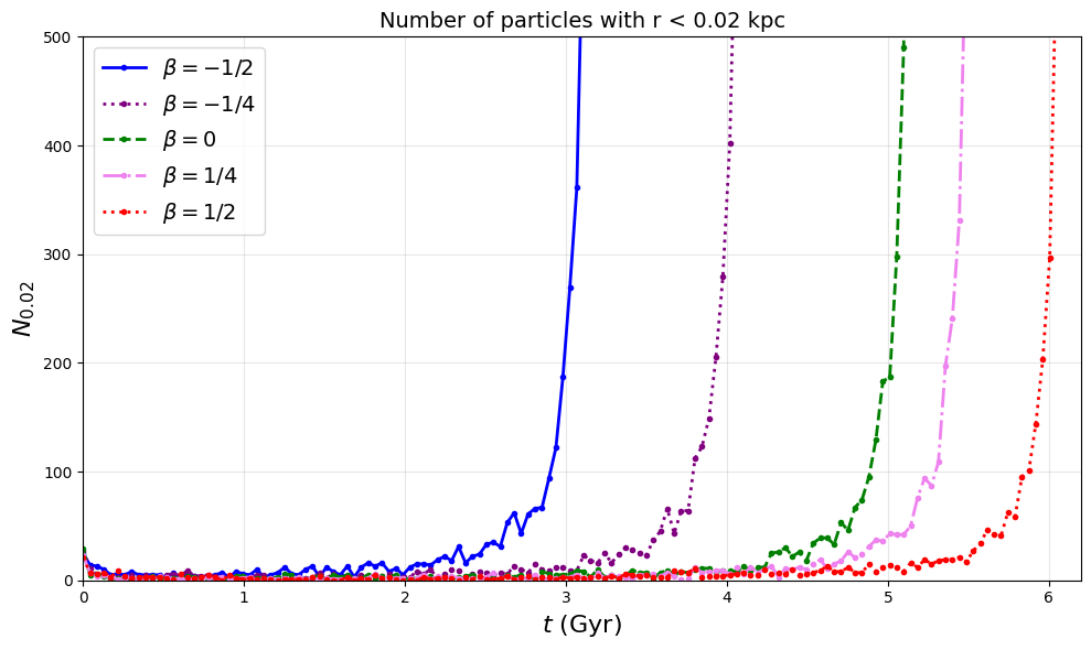
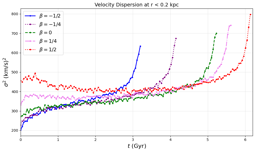
Figures 2a, 2b, 2c: Evolution Analysis for 5 Constant-β Models
This cell analyzes the time evolution of:
Fig 2a: Particle count in innermost 0.02 kpc
Fig 2b: Velocity dispersion in inner 0.2 kpc
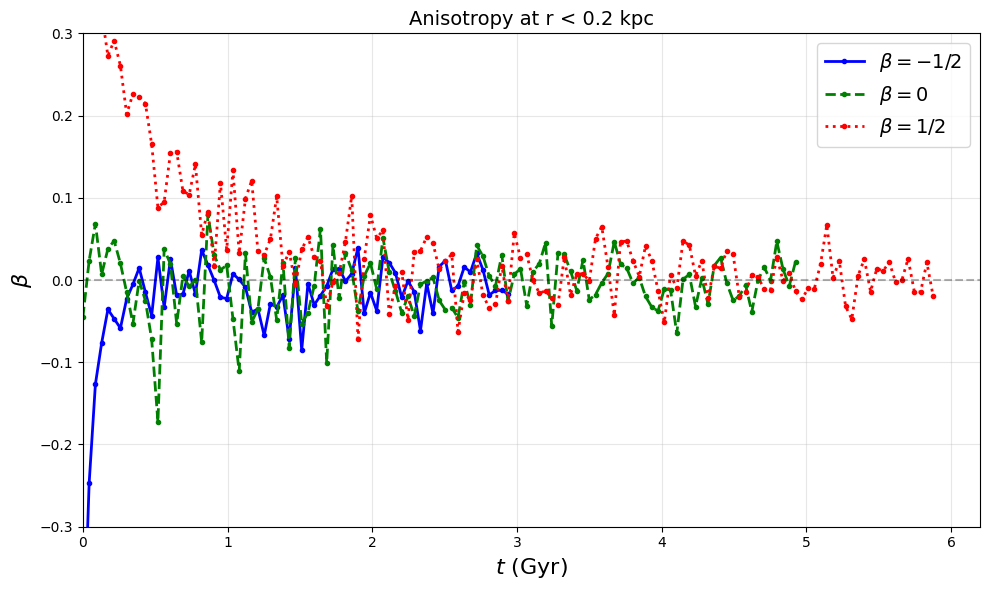
Fig 2c: Anisotropy parameter β evolution
[2]:
from scipy.ndimage import gaussian_filter1d
import numpy as np
import os

record_dtype = np.dtype([
    ('rank',  np.int32),
    ('mass',  np.float32),
    ('R',     np.float32),
    ('Vrad',  np.float32),
    ('PsiA',  np.float32),
    ('E',     np.float32),
    ('L',     np.float32)
])

# Define the five beta configurations
beta_configs = {
    r'$\beta=-1/2$': {
        'path_template': "../data/Rank_Mass_Rad_VRad_unsorted_t00{timestep:03d}_beta-0.5_100000_6250001_300.dat",
        'color': 'blue', 'linestyle': '-'
    },
    r'$\beta=-1/4$': {
        'path_template': "../data/Rank_Mass_Rad_VRad_unsorted_t00{timestep:03d}_beta-0.25_100000_6250001_300.dat",
        'color': 'purple', 'linestyle': ':'
    },
    r'$\beta=0$': {
        'path_template': "../data/Rank_Mass_Rad_VRad_unsorted_t00{timestep:03d}_beta0.0_100000_6250001_300.dat",
        'color': 'green', 'linestyle': '--'
    },
    r'$\beta=1/4$': {
        'path_template': "../data/Rank_Mass_Rad_VRad_unsorted_t00{timestep:03d}_beta0.25_100000_6250001_300.dat",
        'color': 'violet', 'linestyle': '-.'
    },
    r'$\beta=1/2$': {
        'path_template': "../data/Rank_Mass_Rad_VRad_unsorted_t00{timestep:03d}_beta0.5_100000_6250001_300.dat",
        'color': 'red', 'linestyle': ':'
    }
}

time_steps = range(0, 250, 1)
bin_edges = np.arange(0, 2, 0.02)
results = {}
threshold_particles = None

# Process each beta configuration
for beta_label, config in beta_configs.items():
    print(f"Processing {beta_label}...")

    lowest_bin_counts = []
    msv_bins1_n_list = []
    beta_bins1_n_list = []
    actual_time_steps = []

    for time_step in time_steps:
        file_path = config['path_template'].format(timestep=time_step)
        try:
            if not os.path.exists(file_path):
                continue

            alldata = np.fromfile(file_path, dtype=record_dtype)

            if threshold_particles is None and alldata.size > 0:
                threshold_particles = alldata.size / 1000
                print(f"  0.1% threshold = {threshold_particles:.1f} particles (N={alldata.size})")

            if alldata.size == 0:
                continue

            radii = alldata['R']
            vrad = alldata['Vrad']
            L = alldata['L']

            # Calculate tangential velocity
            with np.errstate(divide='ignore', invalid='ignore'):
                vtangential = np.where(radii > 1e-6, L / radii, 0.0)

            # Filter for valid particles
            valid_mask = (np.isfinite(radii) & np.isfinite(vrad) &
                         np.isfinite(vtangential) & (radii > 1e-6))

            if not np.any(valid_mask):
                continue

            radii = radii[valid_mask]
            vrad = vrad[valid_mask]
            vtangential = vtangential[valid_mask]

            # Histogram and smoothing
            counts, _ = np.histogram(radii, bins=bin_edges)
            smoothed_counts = gaussian_filter1d(counts, sigma=0.001)
            lowest_bin_counts.append(smoothed_counts[0])

            # Velocity dispersion for inner bins
            bin_indices = np.digitize(radii, bin_edges, right=False)
            mask_bins1_n = (bin_indices >= 1) & (bin_indices <= 10)
            vrad_bins1_n = vrad[mask_bins1_n]
            vtangential_bins1_n = vtangential[mask_bins1_n]

            if len(vrad_bins1_n) > 10:
                mean_vr2 = np.mean(vrad_bins1_n**2) / (1.023e-3**2)
                mean_vtan2 = np.mean(vtangential_bins1_n**2) / (1.023e-3**2)
                msv_bins1_n = mean_vr2 + mean_vtan2

                # Calculate beta
                if mean_vr2 > 1e-10:
                    beta_bins1_n = 1.0 - mean_vtan2 / (2.0 * mean_vr2)
                    beta_bins1_n = np.clip(beta_bins1_n, -1.0, 1.0)
                else:
                    beta_bins1_n = np.nan
            else:
                msv_bins1_n = np.nan
                beta_bins1_n = np.nan

            msv_bins1_n_list.append(msv_bins1_n)
            beta_bins1_n_list.append(beta_bins1_n)
            actual_time_steps.append(time_step)

        except Exception as e:
            continue

    # Convert to Gyr
    actual_time_steps_gyr = 10.801 / 250 * np.array(actual_time_steps)
    lowest_bin_counts_array = np.array(lowest_bin_counts)

    # Find peak
    if len(lowest_bin_counts_array) > 0:
        max_idx = np.argmax(lowest_bin_counts_array)
    else:
        max_idx = 0

    results[beta_label] = {
        'time': actual_time_steps_gyr[:max_idx+1],
        'time_full': actual_time_steps_gyr,
        'lowest_bin_counts': lowest_bin_counts_array[:max_idx+1],
        'lowest_bin_counts_full': lowest_bin_counts_array,
        'msv_bins1_n': np.array(msv_bins1_n_list)[:max_idx+1],
        'beta_bins1_n': np.array(beta_bins1_n_list),
        'color': config['color'],
        'linestyle': config['linestyle']
    }

print(f"\nProcessed {len(results)} runs")
Processing $\beta=-1/2$...
  0.1% threshold = 100.0 particles (N=100000)
Processing $\beta=-1/4$...
Processing $\beta=0$...
Processing $\beta=1/4$...
Processing $\beta=1/2$...

Processed 5 runs
[3]:
# Figure 2a: Particle count evolution
fig2a, ax2a = plt.subplots(figsize=(10, 6))
for beta_label, data in results.items():
    ax2a.plot(data['time'], data['lowest_bin_counts'],
             marker='.', linestyle=data['linestyle'], color=data['color'],
             label=beta_label, linewidth=2)

ax2a.set_xlabel(r"$t$ (Gyr)", fontsize=16)
ax2a.set_ylabel(r"$N_{0.02}$", fontsize=16)
ax2a.set_title("Number of particles with r < 0.02 kpc", fontsize=14)
ax2a.legend(fontsize=14, loc='best')
ax2a.set_xlim(0, 6.2)
ax2a.set_ylim(0, 500)
ax2a.grid(True, alpha=0.3)
plt.tight_layout()

# Save Figure 2a as PDF (matching paper figure)
# This generates pdf/fig2a.pdf - particle count evolution in central 0.02 kpc
# Comment out the lines below if you only want to view the figure without saving
os.makedirs("pdf", exist_ok=True)
plt.savefig("pdf/fig2a.pdf", dpi=300, bbox_inches='tight')
print('Saved: pdf/fig2a.pdf')

plt.show()
Saved: pdf/fig2a.pdf
[4]:
# Figure 2b: Velocity dispersion evolution - truncate at σ² peak
fig2b, ax2b = plt.subplots(figsize=(10, 6))
for beta_label, data in results.items():
    valid_msv = ~np.isnan(data['msv_bins1_n'])
    if np.any(valid_msv):
        msv_peak_idx = np.argmax(data['msv_bins1_n'][valid_msv])
        ax2b.plot(data['time'][valid_msv][:msv_peak_idx+1],
                 data['msv_bins1_n'][valid_msv][:msv_peak_idx+1],
                 marker='.', linestyle=data['linestyle'], color=data['color'],
                 label=beta_label, linewidth=2)

ax2b.set_xlabel(r"$t$ (Gyr)", fontsize=16)
ax2b.set_ylabel(r'$\sigma^2$ (km/s)$^2$', fontsize=16)
ax2b.set_title("Velocity Dispersion at r < 0.2 kpc", fontsize=14)
ax2b.legend(fontsize=14, loc='best')
ax2b.set_xlim(0, 6.2)
ax2b.grid(True, alpha=0.3)
plt.tight_layout()

# Save Figure 2b as PDF (matching paper figure)
# This generates pdf/fig2b.pdf - velocity dispersion evolution in central 0.2 kpc
# Each curve truncated at its σ² peak to avoid post-collapse artifacts
# Comment out the lines below if you only want to view the figure without saving
os.makedirs("pdf", exist_ok=True)
plt.savefig("pdf/fig2b.pdf", dpi=300, bbox_inches='tight')
print('Saved: pdf/fig2b.pdf')

plt.show()
Saved: pdf/fig2b.pdf
[5]:
# Figure 2c: Beta evolution - truncate at 0.1% threshold (collapse time)
fig2c, ax2c = plt.subplots(figsize=(10, 6))

paper_betas = [r'$\beta=-1/2$', r'$\beta=0$', r'$\beta=1/2$']

for beta_label, data in results.items():
    if beta_label in paper_betas:
        full_counts = data.get('lowest_bin_counts_full', [])
        time_full = np.array(data['time_full'])

        if len(full_counts) > 0 and len(time_full) > 0:
            threshold_mask = full_counts >= threshold_particles
            if np.any(threshold_mask):
                threshold_idx = np.argmax(threshold_mask)
                collapse_time = time_full[threshold_idx]
            else:
                collapse_time = time_full[-1]
        elif len(data['time']) > 0:
            collapse_time = data['time'][-1]
        else:
            continue

        valid_beta = ~np.isnan(data['beta_bins1_n'])
        time_mask = time_full <= collapse_time
        combined_mask = valid_beta & time_mask

        ax2c.plot(time_full[combined_mask], data['beta_bins1_n'][combined_mask],
                 marker='.', linestyle=data['linestyle'], color=data['color'],
                 label=beta_label, linewidth=2)

ax2c.set_xlabel(r"$t$ (Gyr)", fontsize=16)
ax2c.set_ylabel(r'$\beta$', fontsize=16)
ax2c.set_title("Anisotropy at r < 0.2 kpc", fontsize=14)
ax2c.legend(fontsize=14, loc='best')
ax2c.set_xlim(0, 6.2)
ax2c.set_ylim(-0.3, 0.3)
ax2c.grid(True, alpha=0.3)
ax2c.axhline(y=0, color='k', linestyle='--', alpha=0.3)
plt.tight_layout()

# Save Figure 2c as PDF (matching paper figure)
# This generates pdf/fig2c.pdf - anisotropy β evolution for 3 representative runs
# Each curve truncated at 0.1% threshold (when 100 particles enter r < 0.02 kpc)
# Comment out the lines below if you only want to view the figure without saving
os.makedirs("pdf", exist_ok=True)
plt.savefig("pdf/fig2c.pdf", dpi=300, bbox_inches='tight')
print('Saved: pdf/fig2c.pdf')

plt.show()
Saved: pdf/fig2c.pdf
Figures 3a, 3b: Osipkov-Merritt Model Analysis
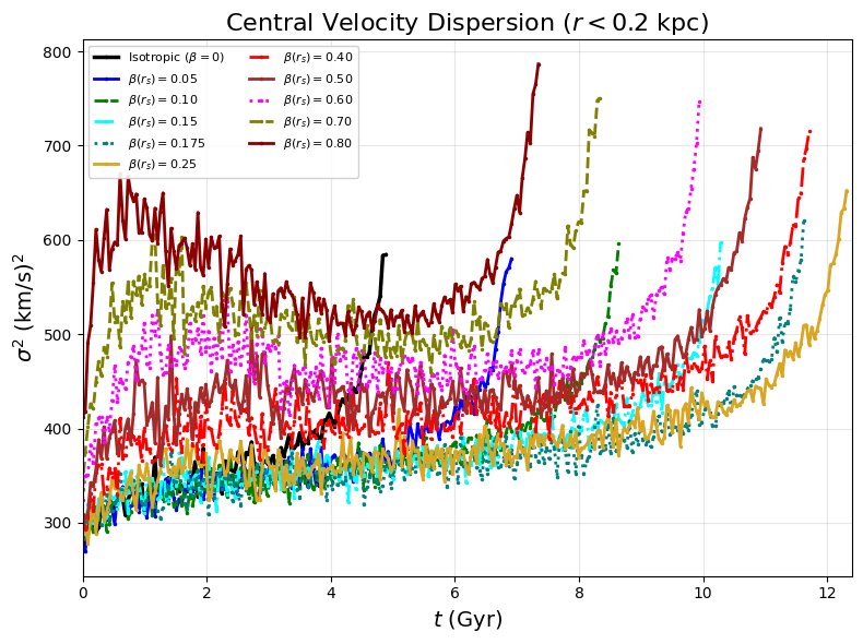
Analyzes 11 Osipkov-Merritt models (isotropic plus 10 anisotropic configurations with β(r_s) from 0.05 to 0.80). Most models use extended runs (ntimesteps=9375001, nout=375, tfinal=450). The isotropic and β(r_s)=0.80 models use standard parameters (ntimesteps=6250001, nout=250, tfinal=300).
These cells create:
Fig 3a: Central velocity dispersion evolution for all OM models
Fig 3b: Core collapse time vs anisotropy parameter β(r_s)
[6]:
# Process OM models - ALL timesteps for each model

import numpy as np
import matplotlib.pyplot as plt
from scipy.ndimage import gaussian_filter1d
import os
import re

kmsec_to_kpcmyr = 1.02271e-3

record_dtype = np.dtype([
    ('rank',  np.int32),
    ('mass',  np.float32),
    ('R',     np.float32),
    ('Vrad',  np.float32),
    ('PsiA',  np.float32),
    ('E',     np.float32),
    ('L',     np.float32)
])

om_configs = {
    r'Isotropic ($\beta=0$)': {
        'path_template': "../data/Rank_Mass_Rad_VRad_unsorted_t00{timestep:03d}_100000_6250001_300.dat",
        'max_t': 250, 'time_factor': 10.801/250,
        'color': 'black', 'linestyle': '-', 'linewidth': 2.5, 'is_om': False
    },
    r'$\beta(r_s)=0.05$': {
        'path_template': "../data/Rank_Mass_Rad_VRad_unsorted_t00{timestep:03d}_betascale0.05_100000_9375001_450.dat",
        'max_t': 375, 'time_factor': 16.2/375,
        'color': 'blue', 'linestyle': '-', 'linewidth': 2, 'is_om': True
    },
    r'$\beta(r_s)=0.10$': {
        'path_template': "../data/Rank_Mass_Rad_VRad_unsorted_t00{timestep:03d}_betascale0.1_100000_9375001_450.dat",
        'max_t': 375, 'time_factor': 16.2/375,
        'color': 'green', 'linestyle': '--', 'linewidth': 2, 'is_om': True
    },
    r'$\beta(r_s)=0.15$': {
        'path_template': "../data/Rank_Mass_Rad_VRad_unsorted_t00{timestep:03d}_betascale0.15_100000_9375001_450.dat",
        'max_t': 375, 'time_factor': 16.2/375,
        'color': 'cyan', 'linestyle': '-.', 'linewidth': 2, 'is_om': True
    },
    r'$\beta(r_s)=0.175$': {
        'path_template': "../data/Rank_Mass_Rad_VRad_unsorted_t00{timestep:03d}_betascale0.175_100000_9375001_450.dat",
        'max_t': 375, 'time_factor': 16.2/375,
        'color': 'teal', 'linestyle': ':', 'linewidth': 2, 'is_om': True
    },
    r'$\beta(r_s)=0.25$': {
        'path_template': "../data/Rank_Mass_Rad_VRad_unsorted_t00{timestep:03d}_betascale0.25_100000_9375001_450.dat",
        'max_t': 375, 'time_factor': 16.2/375,
        'color': 'goldenrod', 'linestyle': '-', 'linewidth': 2, 'is_om': True
    },
    r'$\beta(r_s)=0.40$': {
        'path_template': "../data/Rank_Mass_Rad_VRad_unsorted_t00{timestep:03d}_betascale0.4_100000_9375001_450.dat",
        'max_t': 375, 'time_factor': 16.2/375,
        'color': 'red', 'linestyle': '-.', 'linewidth': 2, 'is_om': True
    },
    r'$\beta(r_s)=0.50$': {
        'path_template': "../data/Rank_Mass_Rad_VRad_unsorted_t00{timestep:03d}_betascale0.5_100000_9375001_450.dat",
        'max_t': 375, 'time_factor': 16.2/375,
        'color': 'brown', 'linestyle': '-', 'linewidth': 2, 'is_om': True
    },
    r'$\beta(r_s)=0.60$': {
        'path_template': "../data/Rank_Mass_Rad_VRad_unsorted_t00{timestep:03d}_betascale0.6_100000_9375001_450.dat",
        'max_t': 375, 'time_factor': 16.2/375,
        'color': 'magenta', 'linestyle': ':', 'linewidth': 2, 'is_om': True
    },
    r'$\beta(r_s)=0.70$': {
        'path_template': "../data/Rank_Mass_Rad_VRad_unsorted_t00{timestep:03d}_betascale0.7_100000_9375001_450.dat",
        'max_t': 375, 'time_factor': 16.2/375,
        'color': 'olive', 'linestyle': '--', 'linewidth': 2, 'is_om': True
    },
    r'$\beta(r_s)=0.80$': {
        'path_template': "../data/Rank_Mass_Rad_VRad_unsorted_t00{timestep:03d}_betascale0.8_100000_6250001_300.dat",
        'max_t': 250, 'time_factor': 10.801/250,
        'color': 'darkred', 'linestyle': '-', 'linewidth': 2, 'is_om': True
    }
}

bin_edges = np.arange(0, 2, 0.02)
results_om = {}
threshold_particles = None

for run_label, config in om_configs.items():
    print(f"Processing {run_label}...")

    lowest_bin_counts = []
    msv_bins1_n_list = []
    actual_times = []

    for t in range(0, config['max_t'] + 1):
        try:
            fpath = config['path_template'].format(timestep=t)
            if not os.path.exists(fpath):
                continue

            data = np.fromfile(fpath, dtype=record_dtype)

            if threshold_particles is None and data.size > 0:
                threshold_particles = data.size / 1000
                print(f"  0.1% threshold = {threshold_particles:.1f} particles")

            if data.size == 0:
                continue

            radii = data['R']
            vrad = data['Vrad']

            valid = np.isfinite(radii) & np.isfinite(vrad) & (radii > 1e-6)
            radii = radii[valid]
            vrad = vrad[valid]

            counts, _ = np.histogram(radii, bins=bin_edges)
            smoothed = gaussian_filter1d(counts, sigma=0.001)
            lowest_bin_counts.append(smoothed[0])

            bin_indices = np.digitize(radii, bin_edges, right=False)
            mask = (bin_indices >= 1) & (bin_indices <= 10)
            vrad_inner = vrad[mask]

            if len(vrad_inner) > 10:
                msv = 3.0 * np.mean(vrad_inner**2) / (1.023e-3**2)
            else:
                msv = np.nan

            msv_bins1_n_list.append(msv)
            actual_times.append(t * config['time_factor'])

        except:
            continue

    print(f"  Processed {len(actual_times)} timesteps")

    results_om[run_label] = {
        'time': np.array(actual_times),
        'msv_bins1_n': np.array(msv_bins1_n_list),
        'lowest_bin_counts_full': np.array(lowest_bin_counts),
        'color': config['color'],
        'linestyle': config['linestyle'],
        'linewidth': config['linewidth'],
        'is_om': config['is_om']
    }

# Calculate threshold times
om_threshold_data = []

for run_label, data in results_om.items():
    if data['is_om']:
        match = re.search(r'beta\(r_s\)=([0-9.]+)', run_label)
        if match:
            beta_s = float(match.group(1))
            counts = data['lowest_bin_counts_full']
            times = data['time']
            threshold_mask = counts >= threshold_particles
            if np.any(threshold_mask):
                om_threshold_data.append({
                    'beta_s': beta_s,
                    't_0.1%': times[np.argmax(threshold_mask)],
                    'color': data['color']
                })

for run_label, data in results_om.items():
    if not data['is_om']:
        counts = data['lowest_bin_counts_full']
        times = data['time']
        threshold_mask = counts >= threshold_particles
        if np.any(threshold_mask):
            om_threshold_data.append({
                'beta_s': 0.0,
                't_0.1%': times[np.argmax(threshold_mask)],
                'color': data['color']
            })

om_threshold_data = sorted(om_threshold_data, key=lambda x: x['beta_s'])
print(f"Processed {len(results_om)} models, {len(om_threshold_data)} cross threshold")
Processing Isotropic ($\beta=0$)...
  0.1% threshold = 100.0 particles
  Processed 251 timesteps
Processing $\beta(r_s)=0.05$...
  Processed 376 timesteps
Processing $\beta(r_s)=0.10$...
  Processed 376 timesteps
Processing $\beta(r_s)=0.15$...
  Processed 376 timesteps
Processing $\beta(r_s)=0.175$...
  Processed 376 timesteps
Processing $\beta(r_s)=0.25$...
  Processed 376 timesteps
Processing $\beta(r_s)=0.40$...
  Processed 376 timesteps
Processing $\beta(r_s)=0.50$...
  Processed 376 timesteps
Processing $\beta(r_s)=0.60$...
  Processed 376 timesteps
Processing $\beta(r_s)=0.70$...
  Processed 376 timesteps
Processing $\beta(r_s)=0.80$...
  Processed 251 timesteps
Processed 11 models, 11 cross threshold
[7]:
# Figure 3a: Central velocity dispersion evolution for all OM models
# Truncate each curve at its velocity dispersion peak
fig_v2, ax_v2 = plt.subplots(figsize=(8, 6))

for run_label, data in results_om.items():
    if len(data['msv_bins1_n']) > 0:
        # Find velocity dispersion peak for THIS curve
        valid_mask = ~np.isnan(data['msv_bins1_n'])
        if np.any(valid_mask):
            msv_valid = data['msv_bins1_n'][valid_mask]
            time_valid = data['time'][valid_mask]

            # Find peak in velocity dispersion
            msv_peak_idx = np.argmax(msv_valid)

            # Plot only up to velocity dispersion peak
            ax_v2.plot(time_valid[:msv_peak_idx+1], msv_valid[:msv_peak_idx+1],
                     marker='.', linestyle=data['linestyle'], color=data['color'],
                     label=run_label, linewidth=data['linewidth'], markersize=3)

ax_v2.set_xlabel(r"$t$ (Gyr)", fontsize=14)
ax_v2.set_ylabel(r"$\sigma^2$ (km/s)$^2$", fontsize=14)
ax_v2.set_title(r"Central Velocity Dispersion ($r < 0.2$ kpc)", fontsize=16)
ax_v2.legend(fontsize=8, loc='upper left', ncol=2, framealpha=0.9)
ax_v2.set_xlim(0, 12.4)
ax_v2.grid(True, alpha=0.3)
ax_v2.tick_params(axis='both', which='major', labelsize=10)
plt.tight_layout()

# Save Figure 3a as PDF (matching paper figure)
# This generates pdf/fig3a.pdf - velocity dispersion for 11 Osipkov-Merritt models
# Each curve shows evolution up to its σ² peak (extended runs to 16.2 Gyr where available)
# Comment out the lines below if you only want to view the figure without saving
os.makedirs("pdf", exist_ok=True)
plt.savefig("pdf/fig3a.pdf", dpi=300, bbox_inches='tight')
print('Saved: pdf/fig3a.pdf')

plt.show()
Saved: pdf/fig3a.pdf
[8]:
# Figure 3b: Core collapse time vs anisotropy parameter
fig_beta, ax_beta = plt.subplots(figsize=(8, 6))

if om_threshold_data:
    beta_s_values = [d["beta_s"] for d in om_threshold_data]
    t_threshold_values = [d["t_0.1%"] for d in om_threshold_data]
    colors = [d["color"] for d in om_threshold_data]

    ax_beta.scatter(beta_s_values, t_threshold_values, c=colors, s=120, zorder=3,
                edgecolors="black", linewidth=1.5, alpha=0.9)
    ax_beta.plot(beta_s_values, t_threshold_values, "k--", alpha=0.3, linewidth=1, zorder=1)

    ax_beta.set_xlabel(r"$\beta(r_s)$", fontsize=14)
    ax_beta.set_ylabel(r"$t_{0.1\%}$ (Gyr)", fontsize=14)
    ax_beta.set_title(r"Core Collapse Time vs Anisotropy", fontsize=16)
    ax_beta.grid(True, alpha=0.3)
    ax_beta.set_xlim(-0.05, max(beta_s_values) + 0.05 if beta_s_values else 0.85)
    ax_beta.axvline(x=0, color="gray", linestyle=":", alpha=0.3)
    ax_beta.tick_params(axis="both", which="major", labelsize=10)

plt.tight_layout()

# Save Figure 3b as PDF (matching paper figure)
# This generates pdf/fig3b.pdf - collapse time (t_0.1%) vs β(r_s) for 11 OM models
# Shows when 100 particles (0.1% threshold) first enter r < 0.02 kpc
# Comment out the lines below if you only want to view the figure without saving
os.makedirs("pdf", exist_ok=True)
plt.savefig("pdf/fig3b.pdf", dpi=300, bbox_inches='tight')
print('Saved: pdf/fig3b.pdf')

plt.show()
Saved: pdf/fig3b.pdf
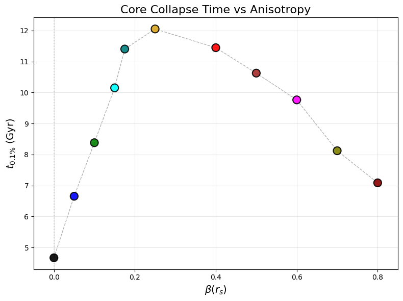
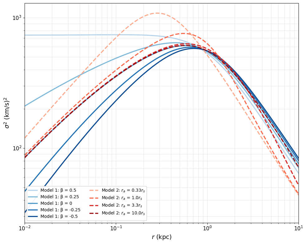
Figure 4: Theoretical Velocity Dispersion Profiles
This cell calculates theoretical velocity dispersion profiles using the Jeans equation. No simulation data required - purely analytical calculations for:
Model 1: Constant β (5 values: -0.5, -0.25, 0, 0.25, 0.5)
Model 2: Osipkov-Merritt with variable β(r) (4 r_a values)
[9]:
import numpy as np
import matplotlib.pyplot as plt
from scipy.integrate import quad
import matplotlib as mpl

# Set up for publication quality
mpl.rcParams['font.size'] = 12
mpl.rcParams['axes.labelsize'] = 14
mpl.rcParams['xtick.labelsize'] = 12
mpl.rcParams['ytick.labelsize'] = 12
mpl.rcParams['legend.fontsize'] = 10
mpl.rcParams['figure.figsize'] = (10, 8)
mpl.rcParams['lines.linewidth'] = 2

# Physical constants
G = 4.302e-6  # kpc (km/s)^2 / M_sun
r_s = 1.18  # kpc
rho_s = 2.73e7  # M_sun / kpc^3

print('Constants:')
print(f'  G = {G} kpc (km/s)^2 / M_sun')
print(f'  r_s = {r_s} kpc')
print(f'  rho_s = {rho_s} M_sun / kpc^3')

# Define functions for Hernquist profile
def M(r):
    """Enclosed mass function"""
    return 2 * np.pi * rho_s * r_s**3 * r**2 / (r**2 + r_s**2)

def n(r):
    """Number density function"""
    return 1 / ((r/r_s) * (1 + r/r_s)**3)

# Model 1: Constant beta
def integrand_model1(r_prime, r, beta):
    """Integrand for model 1"""
    return r_prime**(2*beta - 2) * n(r_prime) * M(r_prime)

def v_r_squared_model1(r, beta):
    """Radial velocity dispersion squared for model 1"""
    integral, _ = quad(integrand_model1, r, np.inf, args=(r, beta))
    return G * integral / (r**(2*beta) * n(r))

def v_squared_model1(r, beta):
    """Total velocity dispersion squared for model 1"""
    return v_r_squared_model1(r, beta) * (3 - 2*beta)

# Model 2: Variable beta (Osipkov-Merritt)
def beta_model2(r, r_a):
    """Beta function for model 2"""
    return r**2 / (r**2 + r_a**2)

def integrand_model2(r_prime, r, r_a):
    """Integrand for model 2"""
    return ((r_a/r_prime)**2 + 1) * n(r_prime) * M(r_prime)

def v_r_squared_model2(r, r_a):
    """Radial velocity dispersion squared for model 2"""
    integral, _ = quad(integrand_model2, r, np.inf, args=(r, r_a))
    return G * integral / ((r_a**2 + r**2) * n(r))

def v_squared_model2(r, r_a):
    """Total velocity dispersion squared for model 2"""
    beta_r = beta_model2(r, r_a)
    return v_r_squared_model2(r, r_a) * (3 - 2*beta_r)

print('Functions defined:')
print('  Model 1 (constant β): v_squared_model1(r, beta)')
print('  Model 2 (OM): v_squared_model2(r, r_a)')

# Create the plot
print('\nGenerating velocity dispersion profiles...')

fig, ax = plt.subplots(1, 1, figsize=(10, 8))

# Radius range (in kpc)
r_range = np.logspace(-2, 1, 100)  # 0.01 to 10 kpc

# Model 1: Plot for different beta values
beta_values = [0.5, 0.25, 0, -0.25, -0.5]
colors_model1 = plt.cm.Blues(np.linspace(0.3, 0.9, len(beta_values)))

print(f'\nModel 1: Computing {len(beta_values)} constant-β profiles...')
for beta, color in zip(beta_values, colors_model1):
    v2_values = [v_squared_model1(r, beta) for r in r_range]
    ax.plot(r_range, v2_values, color=color,
            label=f'Model 1: β = {beta}',
            linestyle='-', linewidth=2.5)
    print(f'  β = {beta:5.2f}: complete')

# Model 2: Plot for different r_a values
r_a_factors = [0.33, 1.0, 3.3, 10.0]
r_a_values = [factor * r_s for factor in r_a_factors]
colors_model2 = plt.cm.Reds(np.linspace(0.3, 0.9, len(r_a_values)))

print(f'\nModel 2: Computing {len(r_a_values)} OM profiles...')
for r_a, factor, color in zip(r_a_values, r_a_factors, colors_model2):
    v2_values = [v_squared_model2(r, r_a) for r in r_range]
    ax.plot(r_range, v2_values, color=color,
            label=f'Model 2: $r_a$ = {factor}$r_s$',
            linestyle='--', linewidth=2.5)
    print(f'  r_a = {factor:4.1f}r_s: complete')

# Formatting with log-log scale
ax.set_xlabel(r'$r$ (kpc)')
ax.set_ylabel(r'$\sigma^2$ (km/s)$^2$')
ax.set_xscale('log')
ax.set_yscale('log')
ax.grid(True, alpha=0.3, which='both')
ax.set_xlim(0.01, 10)

# Create a two-column legend
ax.legend(ncol=2, loc='lower left', framealpha=0.95)

plt.tight_layout()

# Save Figure 4 as PDF (matching paper figure)
# This generates pdf/fig4.pdf - theoretical velocity dispersion profiles from Jeans equation
# Model 1: 5 constant-β profiles (blue solid lines)
# Model 2: 4 Osipkov-Merritt profiles with variable β(r) (red dashed lines)
# Comment out the lines below if you only want to view the figure without saving
os.makedirs("pdf", exist_ok=True)
plt.savefig("pdf/fig4.pdf", dpi=300, bbox_inches='tight')
print('\nSaved: pdf/fig4.pdf')

plt.show()
Constants:
  G = 4.302e-06 kpc (km/s)^2 / M_sun
  r_s = 1.18 kpc
  rho_s = 27300000.0 M_sun / kpc^3
Functions defined:
  Model 1 (constant β): v_squared_model1(r, beta)
  Model 2 (OM): v_squared_model2(r, r_a)

Generating velocity dispersion profiles...

Model 1: Computing 5 constant-β profiles...
  β =  0.50: complete
  β =  0.25: complete
  β =  0.00: complete
  β = -0.25: complete
  β = -0.50: complete

Model 2: Computing 4 OM profiles...
  r_a =  0.3r_s: complete
  r_a =  1.0r_s: complete
  r_a =  3.3r_s: complete
  r_a = 10.0r_s: complete

Saved: pdf/fig4.pdf